Explaining the decisions of machine learning algorithms

Being both statistician and machine learning practitioner, I have always been interested in combining the predictive power of (black box) machine learning algorithms and the interpretability of statistical models.

I thought the only way to combine predictive power and interpretability is by using methods that are somewhat in the middle between 'easy to understand' and 'flexible enough', like decision trees or the RuleFit algorithm or, additionally, by using techniques like partial dependency plots to understand the influence of single features. Then I read the paper "Why Should I Trust You" Explaining the Predictions of Any Classifier [1], which offers a really decent alternative for explaining decisions made by black boxes.

What is LIME?

The authors propose LIME, an algorithm for Local Interpretable Model-agnostic Explanations. LIME can explain why a black box algorithm assigned a specific classification/prediction to one datapoint (image/text/tabular data) by approximating the black box algorithm locally with an interpretable model.

Why was the husky classified as a wolf?

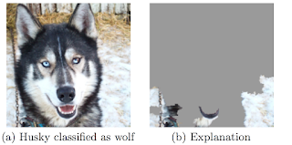
The trustworthiness of an image classifier trained on the task 'Husky vs Wolf' is analysed, as an example in the paper [1]. As a practitioner, you want to check individual false classifications and understand why the classifier went wrong. You can use LIME to approximate and visualize why a husky was classified as a wolf. It turns out that the snow in the image was used to classify the image as 'wolf'. In this case it could help to add more huskies with snow in the background to your training set and more wolfs without snow.

Figure from LIME paper [1]: The husky was mistakenly classified as wolf,
because the classifier learned to use snow as feature.

How LIME works

First you train your algorithm on your classification/prediction task, just as you would usually do. It does not matter if you use a deep neural network or boosted trees, LIME is model-agnostic.

With LIME you can then start to explore explanations for single data points. It works for images, texts and tabular input. LIME creates variations of the data point that you want to have explained. In the case of images, it first splits your image into superpixels and creates new images by randomly switching on and off some of the superpixels. For text it creates versions of the text with some of the words removed. For tabular data the features of the data point are perturbed, to get variations of the data point that are close to the original one. Note that even if you have trained your classifier on a different representation of your data, like bag-of-ngrams or transformations of your original image, you still use LIME on the original data. By creating new variations of your input you create a new dataset (let's call it local interpretable features), where each row represents a perturbation of your input and each column the (interpretable) features (like superpixel). The entries in this datasets are 1 if the superpixel/word was turned on and 0 if it was turned off in a sample. For tabular data the entries are the perturbed values of the features.

LIME puts all those variations through the black box algorithm and gets the predictions. Now the corresponding local interpretable features (e.g. superpixels switched on/off) are used to predict the corresponding output of the black box algorithm. A good choice of model for this job is LASSO, because it will yield a sparse model (e.g. only a few superpixel might be important for the classification). LIME chooses the K best features which then are returned as explanation. For images, each local interpretable feature represents a superpixel and K features are a combination of the best superpixels. For text, each local interpretable feature represents a word and K features are the most important words for the prediction of the black box. In case of tabular data, K features are the columns that contributed most to the prediction.

Why does it work?

The decision boundaries of machine learning algorithms (like neural networks, forests and SVMs) are usually very complex and cannot be comprehended. This changes when you zoom in to one example of your data. The local decision function might be very simple and you can try to approximate it with an interpretable model, like a linear model (LASSO) or a decision tree. Your local classifier has to be faithful, meaning it should reflect the outcome of the black box algorithm closely, otherwise you will not get correct explanations.

Figure from LIME paper [1]: Toy example for decision boundaries of
a classifier. Blue/red represent different classes. The points are perturbed
examples.The line shows the local decision boundary learned
by LIME for the highlighted data point. 

Why is this important?

As machine learning is used in more and more products and processes, it is crucial to have a way of analysing the decision making processes of the algorithms and also to build up trust with the interacting humans.
I predict we will see a future with a lot more machine learning algorithms integrated in every aspect of our life and, coming with that, also regulation and assessments for algorithms, especially in the health, legal and financial industries

What next?

Read the paper: https://arxiv.org/abs/1602.04938
Try out the LIME with Python (only works for text and tabular data at the moment): https://github.com/marcotcr/lime
I have a prototype for the images here: https://github.com/christophM/explain-ml


[1] Ribeiro, M et. al, 2016,  "Why Should I Trust You" Explaining the Predictions of Any Classifier. https://arxiv.org/abs/1602.04938

My first deep learning steps with Google and Udacity

I did my first steps in deep learning by taking the deep learning course at Udacity.

Deep learning is a hot topic. Deep neural networks can classify images, describe scenes, translate text and do so much more. It's great that Google and Udacity offer this course which helped me getting started with learning about deep learning.

Image originally shows me hiking in Switzerland.
Deep neural networks at  Deep Dream Generator turned the image into a dreamy scene.

How does the course work?

The course consists of dozens 1-2 minute videos and assignments accompanying the videos.

Well, actually it's the other way round: The assignments are the heart of the course and the videos just give you the basic understanding you need to get started building networks. There are no exams.

The course covers basic neural networks, softmax, stochastic gradient descent, backpropagation, ReLU units, hidden layers, regularization, dropout, convolutional networks, recurrent networks, LSTM cells and more. Building deep neural networks is a bit like playing Legos and the course shows you the building bricks and teaches you how to use them.

In the assignments you build and optimize deep neural networks that read hand-written letters from images, learn the meaning of words (a la word2vec), can produce texts and flip words in sentences. The assignments are all based on Google's Tensorflow open source library.

The course is extremely hands-on and not self contained. The videos are short with a length of only 1-2 minutes. This concept is very different from the 10-15 minute videos you have in most coursera MOOCs covering all the needed materials. Udacity's deep learning course just gives you an intuitive understanding of the concepts. I found myself reading a lot of other blogs and tutorials to get a better understanding of the course contents and to know enough for the assignments.  I encourage you to read the papers that are linked in the assignments. They are well written and help you to get the assignments done.

I found the explanations in the videos of high quality. They often visualize the concepts and they did a good job at abstracting the concepts.

The assignments can be a bit difficult and you should expect to work a lot on them. Fortunately you can get help in the course forum and also help your peers. I found the community to be very friendly and helpful.

What prior knowledge is needed?

I agree with the prerequisites listed by Udacity: You should have at least 2 years of programming experience, ideally in Python, and you should be able to fork and pull the TensorFlow git repository from Github. The course requires some knowledge in mathematics (matrix multiplication, differentiation, integration and partial derivatives), basic statistics (mean, variance, standard deviation) and basic machine learning concepts. Prior experience with TensorFlow isn't needed. Experience in working with image or text data is also not necessary.

I think you should feel comfortable to read scientific papers, since the assignments encourage you to do so.

All deep neural networks in the assignments can be done with CPUs of most newer laptops (I used an MacBook Pro 13', 2014 model).

The course is self-paced and took me roughly 2.5 months and  4 - 8 hours per week to finish.

Should you take the course?

Yes, given you want to get first hands-on experience in deep learning and/or want to learn TensorFlow. 

Overall the course was fun and I learned a lot.  Even if I am not a big fan of the short videos concept. I wished the videos were a bit longer and had more content.

If you want to do a hands-on MOOC in deep learning there are no other options. For learning the fundamentals you can take coursera Machine Learning class or Neural Networks for Machine Learning.

For me attending the deep learning course lowered the barrier to get into deep learning and I am excited to start building my own deep neural networks.

dplyr is my favourite package for data manipulation.

At my workplace I organized a short dplyr workshop, which I want to share in this blog post.

If you are also interested in learning dplyr and drastically improve readability of your code, you can try out the workshop! The dplyr introduction is followed by some exercises with toy data.

dplyr workshop

The dplyr package

Package for data manipulation. It provides the ‘verbs’ that can be chained together.

Motivation for dplyr

• Fast
• Offers a consistent “grammar”
• Easy to read code, close to language
• It abstracts the data: Can be data.frame, sql

Functionality

• Five basic verbs: filter, select, mutate, arrange, summarise
• Grouping of data
• Joins
• Window functions
• Chains

Verbs

Example: filter(visits, treatment=='a')

• First argument is always the data.frame
• Subsequent arguments describe what to do with the data
• Columns can be used without $
• Return value is the changed data.frame
• filter() to keep the rows that match given criteria
• select() for selecting columns
• mutate() for changing or creating variables
• arrange() reorder rows
• summarise() for summarising a data.frame
• These are the most important verbs, but there are a few more

Chaining with %>%

Example: visits %>% filter(treatment=='a') %>% select(time)

• Verbs can be chained together with %>%
• The outcome from the left hand side of %>% is used as first argument of the function on the right hand side
• The verbs are powerful in combination with the group_by() function

Grouping with group_by()

Example: visits %>% group_by(patient_id) %>% mutate(mean_activity = mean(disease_activity))

• Only useful in conjunction with other verbs
• Returns a special grouped data.frame
• select() not affected
• arrange() orders first by the grouping variable
• mutate() and filter() are done within the groups, useful in conjunction with window function like lag() or mean()
• summarise() summarises for each group
• ungroup() can be used to revert the group_by()

Data

Toy data about patient visits, containing the id of the patients, time of visits, the treatment they receive and a measure of how active the disease is. Just copy-paste the data into an R script and get started with the tasks!

library('dplyr')
visits <- data.frame(patient_id = c(2,2,2,1,1,1,3,4,4,4,4), 
                     time = c(4,2,1,1,2,3,1,2,3,5,4), 
                     treatment = c('a', 'a', 'a', 'b', 'b', 'b', 'c', 'b', 'b', 'b', 'b'), 
                     disease_activity = c(3, 2, 10, 5, 5, 5, 1, 5, 4, 3, 3))

visits 

##    patient_id time treatment disease_activity
## 1           2    4         a                3
## 2           2    2         a                2
## 3           2    1         a               10
## 4           1    1         b                5
## 5           1    2         b                5
## 6           1    3         b                5
## 7           3    1         c                1
## 8           4    2         b                5
## 9           4    3         b                4
## 10          4    5         b                3
## 11          4    4         b                3

Tasks

Solve the following tasks using the dplyr package. The desired output is displayed. For revealing the solution, click ‘Show Code’. But try it yourself first. ;-)

Filter (=keep rows of) patients who got treatment a or b

filter(visits, treatment %in% c('a', 'b'))

##    patient_id time treatment disease_activity
## 1           2    4         a                3
## 2           2    2         a                2
## 3           2    1         a               10
## 4           1    1         b                5
## 5           1    2         b                5
## 6           1    3         b                5
## 7           4    2         b                5
## 8           4    3         b                4
## 9           4    5         b                3
## 10          4    4         b                3

Sort visits by patient id and time

arrange(visits, patient_id, time)

##    patient_id time treatment disease_activity
## 1           1    1         b                5
## 2           1    2         b                5
## 3           1    3         b                5
## 4           2    1         a               10
## 5           2    2         a                2
## 6           2    4         a                3
## 7           3    1         c                1
## 8           4    2         b                5
## 9           4    3         b                4
## 10          4    4         b                3
## 11          4    5         b                3

Add column ‘disease activity higher or equal than 4’ (TRUE / FALSE)

mutate(visits, high_disease_activity = disease_activity >= 4)

##    patient_id time treatment disease_activity high_disease_activity
## 1           2    4         a                3                 FALSE
## 2           2    2         a                2                 FALSE
## 3           2    1         a               10                  TRUE
## 4           1    1         b                5                  TRUE
## 5           1    2         b                5                  TRUE
## 6           1    3         b                5                  TRUE
## 7           3    1         c                1                 FALSE
## 8           4    2         b                5                  TRUE
## 9           4    3         b                4                  TRUE
## 10          4    5         b                3                 FALSE
## 11          4    4         b                3                 FALSE

Remove column disease_activity

select(visits, -disease_activity)

##    patient_id time treatment
## 1           2    4         a
## 2           2    2         a
## 3           2    1         a
## 4           1    1         b
## 5           1    2         b
## 6           1    3         b
## 7           3    1         c
## 8           4    2         b
## 9           4    3         b
## 10          4    5         b
## 11          4    4         b

Rename column time to year_since_inclusion

rename(visits, year_since_inclusion=time)

##    patient_id year_since_inclusion treatment disease_activity
## 1           2                    4         a                3
## 2           2                    2         a                2
## 3           2                    1         a               10
## 4           1                    1         b                5
## 5           1                    2         b                5
## 6           1                    3         b                5
## 7           3                    1         c                1
## 8           4                    2         b                5
## 9           4                    3         b                4
## 10          4                    5         b                3
## 11          4                    4         b                3

How many visits exist per time point?

visits %>%
  group_by(time) %>%
  summarise(n = n())

## Source: local data frame [5 x 2]
## 
##    time     n
##   (dbl) (int)
## 1     1     3
## 2     2     3
## 3     3     2
## 4     4     2
## 5     5     1

What is the median, minimum and maximum disease activity at the second visit? Time == 2 is not equivalent to the second visit for all patients.

visits %>%
  group_by(patient_id) %>%
  arrange(time) %>%
  filter(row_number() == 2) %>%
  ungroup() %>%
  summarise(median_activity = median(disease_activity), 
            max_activity = max(disease_activity), 
            min_activity = min(disease_activity))

## Source: local data frame [1 x 3]
## 
##   median_activity max_activity min_activity
##             (dbl)        (dbl)        (dbl)
## 1               4            5            2

Sort visits descending by disease activity

arrange(visits, desc(disease_activity))

##    patient_id time treatment disease_activity
## 1           2    1         a               10
## 2           1    1         b                5
## 3           1    2         b                5
## 4           1    3         b                5
## 5           4    2         b                5
## 6           4    3         b                4
## 7           2    4         a                3
## 8           4    5         b                3
## 9           4    4         b                3
## 10          2    2         a                2
## 11          3    1         c                1

Filter patients with treatment c and select the disease activity column

visits %>% 
  filter(treatment == 'c') %>%
  select(disease_activity)

##   disease_activity
## 1                1

Create a new variable per patient: nth visit

visits %>%
  group_by(patient_id) %>%
  mutate(nth_visit = rank(time))

## Source: local data frame [11 x 5]
## Groups: patient_id [4]
## 
##    patient_id  time treatment disease_activity nth_visit
##         (dbl) (dbl)    (fctr)            (dbl)     (dbl)
## 1           2     4         a                3         3
## 2           2     2         a                2         2
## 3           2     1         a               10         1
## 4           1     1         b                5         1
## 5           1     2         b                5         2
## 6           1     3         b                5         3
## 7           3     1         c                1         1
## 8           4     2         b                5         1
## 9           4     3         b                4         2
## 10          4     5         b                3         4
## 11          4     4         b                3         3

Filter all patients with only one visit. Hint: Use n()

visits %>% 
  group_by(patient_id) %>% 
  filter(n() == 1)

## Source: local data frame [1 x 4]
## Groups: patient_id [1]
## 
##   patient_id  time treatment disease_activity
##        (dbl) (dbl)    (fctr)            (dbl)
## 1          3     1         c                1

Calculate the change of disease activity per visit for each patient. Also the change over two visits. Hint: Use lag()

visits %>% 
  group_by(patient_id) %>% 
  arrange(time) %>%
  mutate(change = disease_activity - lag(disease_activity), 
         change_2 = disease_activity - lag(disease_activity, n=2)) 

## Source: local data frame [11 x 6]
## Groups: patient_id [4]
## 
##    patient_id  time treatment disease_activity change change_2
##         (dbl) (dbl)    (fctr)            (dbl)  (dbl)    (dbl)
## 1           1     1         b                5     NA       NA
## 2           1     2         b                5      0       NA
## 3           1     3         b                5      0        0
## 4           2     1         a               10     NA       NA
## 5           2     2         a                2     -8       NA
## 6           2     4         a                3      1       -7
## 7           3     1         c                1     NA       NA
## 8           4     2         b                5     NA       NA
## 9           4     3         b                4     -1       NA
## 10          4     4         b                3     -1       -2
## 11          4     5         b                3      0       -1