Explaining the decisions of machine learning algorithms

Being both statistician and machine learning practitioner, I have always been interested in combining the predictive power of (black box) machine learning algorithms and the interpretability of statistical models.

I thought the only way to combine predictive power and interpretability is by using methods that are somewhat in the middle between 'easy to understand' and 'flexible enough', like decision trees or the RuleFit algorithm or, additionally, by using techniques like partial dependency plots to understand the influence of single features. Then I read the paper "Why Should I Trust You" Explaining the Predictions of Any Classifier [1], which offers a really decent alternative for explaining decisions made by black boxes.

What is LIME?

The authors propose LIME, an algorithm for Local Interpretable Model-agnostic Explanations. LIME can explain why a black box algorithm assigned a specific classification/prediction to one datapoint (image/text/tabular data) by approximating the black box algorithm locally with an interpretable model.

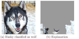
Why was the husky classified as a wolf?

The trustworthiness of an image classifier trained on the task 'Husky vs Wolf' is analysed, as an example in the paper [1]. As a practitioner, you want to check individual false classifications and understand why the classifier went wrong. You can use LIME to approximate and visualize why a husky was classified as a wolf. It turns out that the snow in the image was used to classify the image as 'wolf'. In this case it could help to add more huskies with snow in the background to your training set and more wolfs without snow.

Figure from LIME paper [1]: The husky was mistakenly classified as wolf,
because the classifier learned to use snow as feature.

How LIME works

First you train your algorithm on your classification/prediction task, just as you would usually do. It does not matter if you use a deep neural network or boosted trees, LIME is model-agnostic.

With LIME you can then start to explore explanations for single data points. It works for images, texts and tabular input. LIME creates variations of the data point that you want to have explained. In the case of images, it first splits your image into superpixels and creates new images by randomly switching on and off some of the superpixels. For text it creates versions of the text with some of the words removed. For tabular data the features of the data point are perturbed, to get variations of the data point that are close to the original one. Note that even if you have trained your classifier on a different representation of your data, like bag-of-ngrams or transformations of your original image, you still use LIME on the original data. By creating new variations of your input you create a new dataset (let's call it local interpretable features), where each row represents a perturbation of your input and each column the (interpretable) features (like superpixel). The entries in this datasets are 1 if the superpixel/word was turned on and 0 if it was turned off in a sample. For tabular data the entries are the perturbed values of the features.

LIME puts all those variations through the black box algorithm and gets the predictions. Now the corresponding local interpretable features (e.g. superpixels switched on/off) are used to predict the corresponding output of the black box algorithm. A good choice of model for this job is LASSO, because it will yield a sparse model (e.g. only a few superpixel might be important for the classification). LIME chooses the K best features which then are returned as explanation. For images, each local interpretable feature represents a superpixel and K features are a combination of the best superpixels. For text, each local interpretable feature represents a word and K features are the most important words for the prediction of the black box. In case of tabular data, K features are the columns that contributed most to the prediction.

Why does it work?

The decision boundaries of machine learning algorithms (like neural networks, forests and SVMs) are usually very complex and cannot be comprehended. This changes when you zoom in to one example of your data. The local decision function might be very simple and you can try to approximate it with an interpretable model, like a linear model (LASSO) or a decision tree. Your local classifier has to be faithful, meaning it should reflect the outcome of the black box algorithm closely, otherwise you will not get correct explanations.

Figure from LIME paper [1]: Toy example for decision boundaries of
a classifier. Blue/red represent different classes. The points are perturbed
examples.The line shows the local decision boundary learned
by LIME for the highlighted data point. 

Why is this important?

As machine learning is used in more and more products and processes, it is crucial to have a way of analysing the decision making processes of the algorithms and also to build up trust with the interacting humans.
I predict we will see a future with a lot more machine learning algorithms integrated in every aspect of our life and, coming with that, also regulation and assessments for algorithms, especially in the health, legal and financial industries

What next?

Read the paper: https://arxiv.org/abs/1602.04938
Try out the LIME with Python (only works for text and tabular data at the moment): https://github.com/marcotcr/lime
I have a prototype for the images here: https://github.com/christophM/explain-ml


[1] Ribeiro, M et. al, 2016,  "Why Should I Trust You" Explaining the Predictions of Any Classifier. https://arxiv.org/abs/1602.04938

RuleFit: When disassembled trees meet Lasso

The RuleFit algorithm from Friedman and Propescu is an interesting regression and classification approach that uses decision rules in a linear model.

RuleFit is not a completely new idea, but it combines a bunch of algorithms in a clever way. RuleFit consists of two components: The first component produces "rules" and the second component fits a linear model with these rules as input (hence the name "RuleFit"). The cool thing about the algorithm is that the produced model is highly interpretable, because the decision rules have an easy understandable format, but you still have a flexible enough approach to capture complex interactions and get a good fit.

Part I: Generate rules 

The rules that the algorithm generates have a simple form:

if  x2 < 3  and  x5 < 7  then  1  else  0

The rules are generated from the covariates matrix X. You can also see the rules simply as new features based on your original features.

The RuleFit paper uses the Boston housing data as example: The goal is to predict the median house value in the Boston neighborhood. One of the rules that is generated by RuleFit is:

if  (number of rooms > 6.64)  and  (concentration of nitric oxide < 0.67) then 1 else 0

The interesting part is how those rules are generated: They are derived from Decision Trees, by basically ripping them apart. Every path in a tree can be turned into a decision rule. You simply chain the binary decisions that lead to a certain node et voilà, you have a rule. It is desirable to generate a lot of diverse and meaningful rules. Gradient boosting is used to fit an ensemble of decision trees (by regressing/classifying y with your original features X). Each resulting trees is turned into multiple rules.

4 rules can be generated from a tree with 3 terminal nodes

Another way to see this step is a black box, that generates a new set of features X' out of your original features X. Those features are binary and can represent quite complex interactions of your original X. The rules are chosen to maximise the prediction/classification task at hand.

Part II: Fit the rules

You will get A LOT of rules from the first step (and that is what you want). Since the first step is only a feature transformation function on your original data set you are still not done with fitting a model and also you want to reduce the number of rules. Lasso or L1 regularised regression is good in this scenario. Next to the rules also all numeric variables from your original data set will be used in the Lasso linear model. Every rule and numeric variable gets a coefficient (beta). And thanks to the regularisation, a lot of those betas will be estimated to zero. The numeric variables are added because trees suck at representing simple linear relationships between y and x. The outcome is a linear model that has linear effects for all of the numeric variables and also linear terms for the rules.

The paper not only introduces RuleFit and evaluates it, but it also comes with a bunch of useful tools, (comparable to Random Forest): Measurement tools for variable importance, degree of relevance of original input variables and interaction effects between variables.

There are currently two implementations out there one from the authors in R and one in the TMVA toolkit.

tl;dr  The RuleFit regression and classification algorithm works by boosting an ensemble of decision trees, creating decision rules from those trees and throwing the rules (+ the numeric covariables) at L1 regularized regression (Lasso). Try it out.

Get the party started

Have you already used trees or random forests to model a relationship of a response and some covariates? Then you might like the condtional trees, which are implemented in the party package.

In difference to the CART (Classification and Regression Trees) algorithm, the conditional trees algorithm uses statistical hypothesis tests to determine the next split. Every variable is tested at each splitting step, if it has an association with the response. The variable with the lowest p-value is taken for the next split. This is done until the global null-hypothesis of independence of the response and all covariates can not be rejected.

Conditional trees is my subject in a university seminar this semester. Here are my slides explaining the functionality of conditional trees, which I wanted to share with you. It includes the theory and two short examples in R.

Conditional trees from Christoph Molnar

Trees with the rpart package

What are trees?

Trees (also called decision trees, recursive partitioning) are a simple yet powerful tool in predictive statistics. The idea is to split the covariable space into many partitions and to fit a constant model of the response variable in each partition. In case of regression, the mean of the response variable in one node would be assigned to this node. The structure is similar to a real tree (from the bottom up): there is a root, where the first split happens. After each split, two new nodes are created (assuming we only make binary splits). Each node only contains a subset of the observations. The partitions of the data, which are not split any more, are called terminal nodes or leafs. This simple mechanism makes the interpretation of the model pretty easy.

Interpretation looks like: “If \(x1 > 4\) and \(x2 < 0.5\) than \(y = 12\)." This is much easier to explain to  a non-statistician than a linear model. Therefore it is a powerful tool not only for prediction, but also to explain the relation of your response \(Y\) and your covariables \(X\) in an easy understandable way.

Different algorithms implement these kind of trees. They differ in the criterion, which decides how to split a variable, the number of splits per step and other details. Another difference is how pruning takes places. Pruning means to shorten the tree, which makes trees more compact and avoids overfitting to the training data. The algorithms have in common, that they all use some criterion to decide about the next split. In case of regression, the split criterion is the sum of squares in each partition. The split is made at the variable and split point, where the best split can be achieved according to the criterion (regression trees: minimal sum of squares)

To avoid too large trees, there are two possible methods:

1. Avoid growing large trees: This is also called early stopping. Stopping criteria might be, that the number of observations in a node undercuts some minimum number of observations. If the criterion is fulfilled the current node will not be split any further. Early stopping yields smaller trees and saves computational time.

 2. Grow large tree, cut afterwards: Also known as pruning. The full tree is grown (early stopping might additionally be used), and each split is examined, if it brings a reliable improvement. This can be top-down, starting from the first split made, or bottom-up, starting at the splits above the terminal nodes. Bottom-up is more common, because top-down has the problem, that whole sub-trees can be trashed. However, after a "bad” split a lot of good splits can follow. Pruning takes into account the weighted split criterion for all splits and the complexity of the trees, which is weighted by some \(\alpha\). Normally the complexity parameter \(\alpha\) is chosen data-driven by cross-validation.


How can I use those trees?

The R package rpart implements recursive partitioning. It is very easy to use. The following example uses the iris data set. I'm trying to find a tree, which can tell me if an Iris flower species is setosa, versicolor or virginica, using some measurements as covariables. As the response variable is categorial,  the resulting tree is called classification tree. The default criterion, which is maximized in each split is the gini coefficient. The model, which is fit to each node, is simply the mode of the flower species, the flower which appears most often in this node.

The result is a very short tree: If Petal.length is smaller than 2.4 we label the flower with setosa. Else we look at the covariable Petal.Width. Is Petal.Width smaller than 1.8? If so, we label the flower versicolor, else virginica.

I personally think the plots from the rpart package are very ugly, so I use the plot function rpart.plot from the rpart.plot package. The results from the tree show, that all of the Iris flowers which are in the left node are correctly labeled setosa, no other flower is in this terminal node of the tree. The other terminal nodes are also very pure, the versicolor labeled node contains 54 correctly assigned flowers and 5 wrongly assigned. The virginic node has about the same purity (46 correctly, 1 incorrectly assigned).

library("rpart")
library("rpart.plot")
data("iris")

tree <- rpart(Species ~ ., data = iris, method = "class")
rpart.plot(tree)

tree

## n= 150 
## 
## node), split, n, loss, yval, (yprob)
##       * denotes terminal node
## 
## 1) root 150 100 setosa (0.33333 0.33333 0.33333)  
##   2) Petal.Length< 2.45 50   0 setosa (1.00000 0.00000 0.00000) *
##   3) Petal.Length>=2.45 100  50 versicolor (0.00000 0.50000 0.50000)  
##     6) Petal.Width< 1.75 54   5 versicolor (0.00000 0.90741 0.09259) *
##     7) Petal.Width>=1.75 46   1 virginica (0.00000 0.02174 0.97826) *

The method-argument can be switched according to the type of the response variable. It is “class”“ for categorial, "anova”“ for numerical, "poisson”“ for count data and "exp”“ for survival data.
All in all the package is pretty easy to use. Thanks to the formula interface, it can be used like most other regression models (like lm(), glm() and so on). I personally think the utility of trees as regression models is underestimated. They are super-easy to understand and if you have to work with non-statistician it might be a benefit to use trees.


Further readings:

• Rpart Tutorial 
• Introduction to Trees: Elements of Statistical Learning, page 305 - 310